Building a MovieLens Recommender with Biased Matrix Factorisation

Google Colab notebook: Open in Google Colab · Raw Notebook: Download .ipynb
For this exercise, I developed a recommender system in stages, from simple baselines to biased matrix factorisation, before asking whether SHAP explanations make individual predictions more understandable. What stood out was that better rating prediction did not automatically produce better top-10 ranking.
Data and Method
The notebook downloads MovieLens 100K directly from GroupLens and verifies the archive checksum before loading it. Validation confirmed 100,000 unique user-movie ratings from 943 users across 1,682 films, with no missing fields and ratings restricted to 1–5. MovieLens is deliberately modest, but its stable structure makes it useful for comparing recommender algorithms (Harper and Konstan, 2015).
To avoid training on a user's future, I sorted each user's ratings chronologically. Their earliest 80% formed training data, the next 10% validation data and the latest 10% test data. This produced 79,619 training, 9,942 validation and 10,439 test ratings. Every test user had training history, although 52 test rows involved movies absent from training. Those rows used a bias-only cold-start fallback.
I first calculated the training-set global mean, then fitted regularised user and movie biases. These baselines made it possible to check whether added complexity genuinely improved generalisation rather than merely fitting the training data (Deepchecks, n.d.). The final model estimates a rating as the global mean plus user bias, movie bias and a 20-factor latent interaction. Its parameters were learned with SGD, regularisation and validation monitoring, following the collaborative-filtering progression discussed by Theobald (2024).
Results and Diagnostics
The executed test-set comparison shows how much each modelling stage reduced rating error. Lower values are better for both metrics.
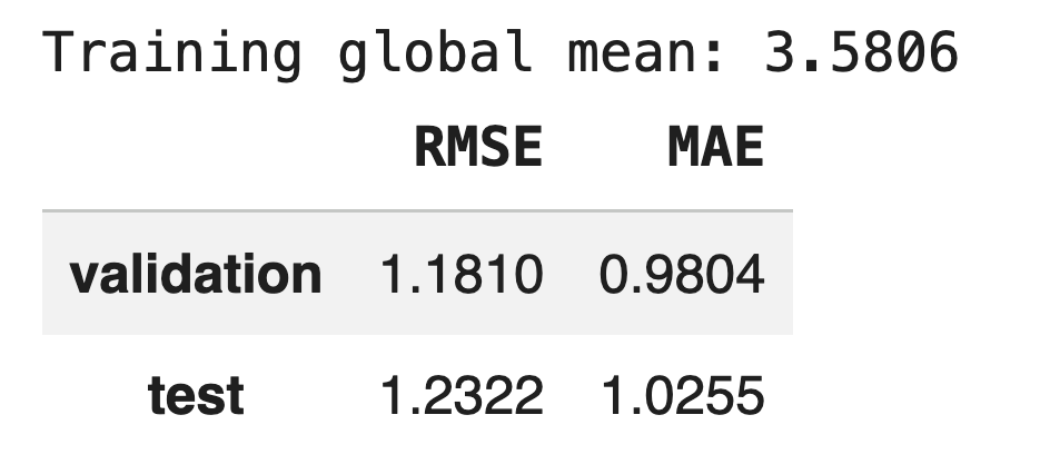
Matrix factorisation improved RMSE by about 2.9% over the strong bias baseline. Its known-user/known-movie RMSE was 0.9857, while the cold-movie fallback reached 1.3005. This gap makes the uncertainty around unseen items visible rather than hiding it inside one aggregate score. Test residuals had a mean of −0.0613, indicating slight under-prediction overall.
Ranking told a less flattering story. I treated ratings of 4 or 5 as relevant, excluded movies already seen before the test period, and ranked the remaining catalogue for 856 evaluable users. The macro-averaged comparison at K=10 is shown below; higher values are better.
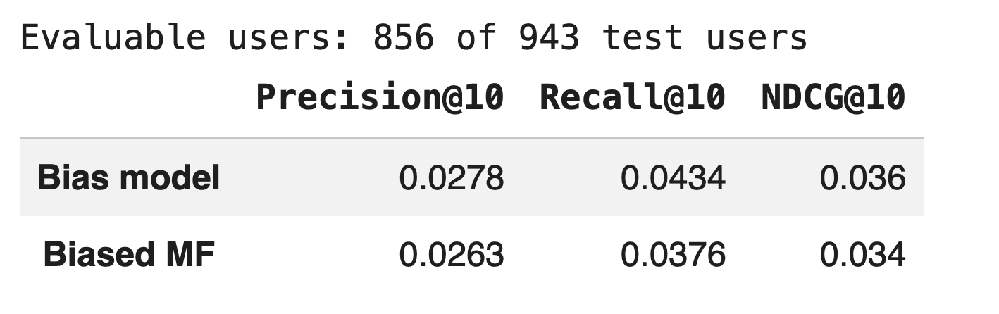
The bias model led on precision, recall and NDCG. Matrix factorisation therefore predicted rating values more accurately but did not improve the recommendation ordering. This result shows why rating prediction and recommendation ranking must be evaluated separately: a model optimised for squared rating error is not necessarily optimised for top-K discovery, and an unrated film does not necessarily indicate a negative preference.
Does the SHAP Explanation Make Sense?
The latent vectors are difficult to describe to a user. I therefore exposed the matrix-factorisation model's three raw-score components: user bias, movie bias and latent match. They reconstructed the unclipped score exactly, with an R² of 1.0 and MAE of 0. SHAP then expressed how each component moved a prediction away from the background value, consistent with its additive local-explanation design (Lundberg and Lee, 2017).
For user 632, the model predicted 4.60 for Star Wars (1977), whose training mean was 4.35. Movie bias contributed +0.695 and latent match +0.565, while user bias contributed −0.199. For the same user, Leave It to Beaver (1997) was predicted 1.60; its movie bias contributed −1.770 and dominated the explanation. The contrast makes sense as a description of the model and training data. It does not prove that either film is objectively good or that these factors caused the user's preference. The latent-match term remains abstract, and SHAP values depend on the chosen background. Rahim M and Basheer K.P (2025) likewise distinguish local explanations for individual recommendations from aggregated global explanations and stress translating technical attributions for end users.
Critical Reflection
Working in stages kept three questions separate: whether matrix factorisation improved held-out rating prediction, whether it ranked relevant unseen films effectively, and whether SHAP could communicate its scores without implying causation. This prevented the stronger RMSE from obscuring the weaker ranking performance.
The chronological split is more deployment-like than a random split, but one historical MovieLens subset cannot establish current performance. Ranking metrics also rely on the unobserved-feedback assumption noted above, while a plausible SHAP explanation remains a diagnostic rather than proof that the model is correct.
In a development team, data engineers would own validation and lineage, ML engineers the reproducible experiment, product specialists the definition of relevance and error costs, and QA/MLOps colleagues cold-start and drift testing. My role would include reporting the weaker ranking result and explanation limitations alongside the stronger RMSE. Results, limitations and component fidelity should be documented so stakeholders can challenge the recommendations rather than receiving only the model's most favourable metric.
References
Deepchecks (n.d.) ‘Baseline models’. Available at: https://deepchecks.com/glossary/baseline-models/ (Accessed: 11 July 2026).
Harper, F.M. and Konstan, J.A. (2015) ‘The MovieLens datasets: History and context’, ACM Transactions on Interactive Intelligent Systems, 5(4), article 19. Available at: https://doi.org/10.1145/2827872 (Accessed: 11 July 2026).
Lundberg, S.M. and Lee, S.-I. (2017) ‘A unified approach to interpreting model predictions’, Advances in Neural Information Processing Systems, 30. Available at: https://proceedings.neurips.cc/paper_files/paper/2017/hash/8a20a8621978632d76c43dfd28b67767-Abstract.html (Accessed: 11 July 2026).
Rahim M, N. and Basheer K.P, M. (2025) ‘A hybrid explainability framework for recommender systems using SHAP with natural language interpretations’, International Journal of Innovative Research and Scientific Studies, 8(6), pp. 687–703. Available at: https://doi.org/10.53894/ijirss.v8i6.9669 (Accessed: 11 July 2026).
Theobald, O. (2024) Machine Learning: Make Your Own Recommender System. Birmingham: Packt Publishing. Available at: https://www.oreilly.com/library/view/machine-learning-make/9781835882061/ (Accessed: 11 July 2026).